Iris Biometrics

The main strategy for iris recognition is to find the area around the pupil, but inside the sclera. The iris is unique to each individual person, including twins.

Strategy

The general strategy to use this metric is to first find the outside of the iris, then the inside of the region. This resultant image will be a polar coordinate representation of the iris, so we convert it into the Cartesian form, in a format that is much easier for a computer to reason with.

From this image, we can then extract features, and differentiate between people. The texture of an iris is mapped from the visual space into a binary code that belongs to one individual only.

Problems

Iris recognition can be made harder by the lighting, eyebrows, eyelids and other peculiarities such as a white dot from a point light source.

Historically, recognition has been done with an infrared camera, as this has yielded much more detail. Now, we also use cameras in the visible spectrum.

Anatomy

An iris comprises many different features. These can be seen in the image below:

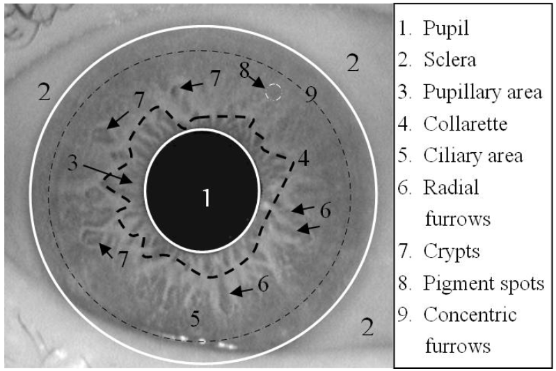
Advantages and Disadvantages

Iris recognition is a completely unique biometric, even down to the individual eye level on the same person. Irises are a stable biometric as they do not change with time, unlike the gait or the face of a person. Iris recognition, similar to gait, is a non-contact biometric.

Initial Approach

The first approaches used near-infrared cameras, in contrast to recent developments which might want to use commonly available technology (e.g., a phone camera).

Detection

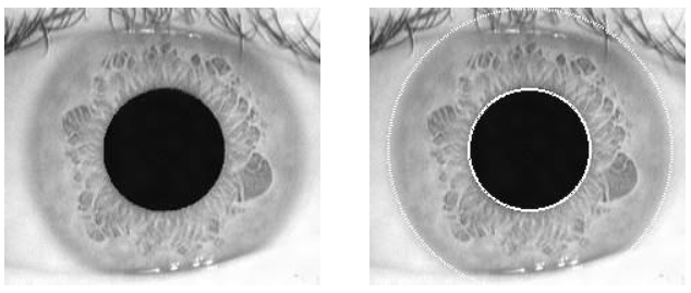
The first method is known as the Daugman Method, IEEE TPAMI, 1993. The strategy here was to detect outer and inner boundaries, then transform from polar to Cartesian.

From here, he transferred from the image to a binary code which is the extracted feature. The main equation is as follows:

\[ \max_{(r, x_0, y_0)} \left| G_\sigma (r) * \frac{\delta}{\delta r} \oint_{r,x_0,y_0} \frac{I(x,y)}{2\pi r} ds \right| \]

Let's break this equation down, and examine what each part of it is responsible for. The initial bit that confused me was the \(\oint\) sign. This simply means that we are taking the integral of a circle, as opposed to a straight line.

So what does the equation actually do? We want to compute the value of an \(r_1\), which is the outer radius of a circle, and \(r_2\), which is the inner radius of a circle. These radii form a doughnut shape on the eye, and the algorithm must be able to find these points without any manual user intervention (this is computer vision after all).

The \(\max_{(r,x_0,y_0)}\) is taking all the outputs from the scary bit on the right, and reducing these outputs to the values of \(r\) that are highest across the circle, given some centre \(x_0,y_0\).

The \(x_0,y_0\) are simply the centre of the circle (recall that the equation for a circle is \((x-x_0)^2 + (y-y_0)^2 = r^2\)).

From here, we can move right. The \(|\)'s either side just take the absolute value of everything internally. Next, the \(I(x,y)\) equation returns the grayscale value of a pixel at \((x,y)\). The \(2\pi r\) term divides this by the perimeter of the circle.

The whole \(\frac{I(x,y)}{2\pi r}\) gets the average of the pixels along the path. Next, we can integrate this and plot increasing \(r\) on the \(x\)-axis, with the integrand on the \(y\) axis. This will help to find unknown \(r\). We calculate for many different values of \(r\), and will yield a plot that looks as follows:

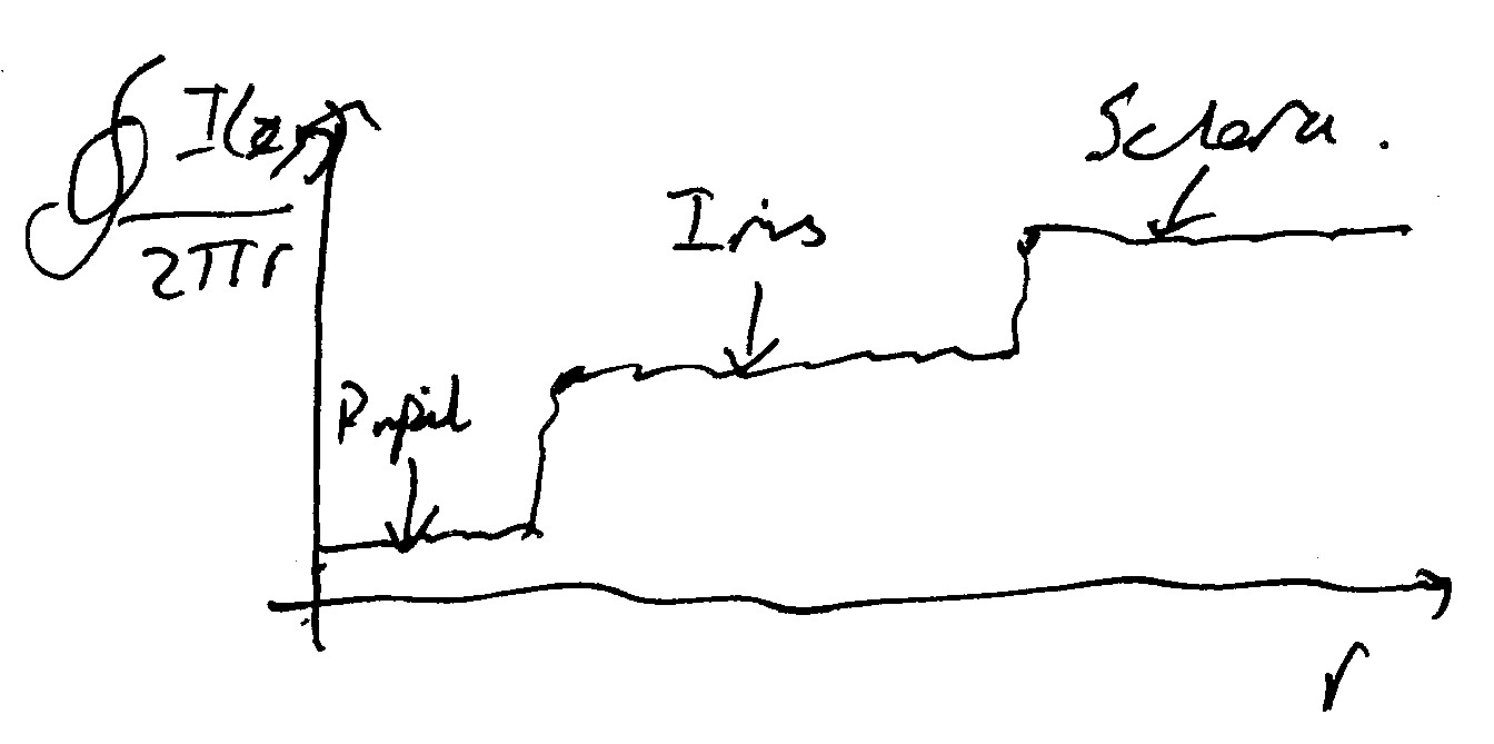
As we can see there, the plot shows initially a low (slightly noisy) region for the pupil, which makes sense as the brightness of the pupil is minimal. From here, we get a jump in the integration, as we begin to work through \(r\) within the iris (this will be from \(r_1\) to \(r_2\)).

After this bit, there will be another jump as we reach the sclera of the eye is reached.

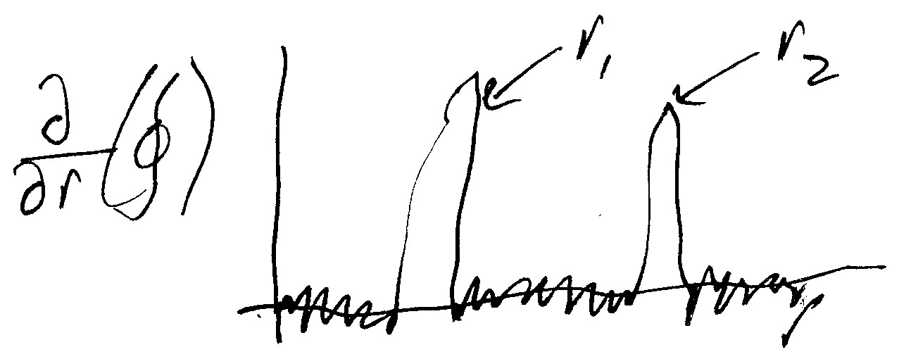
This plot is quite noisy, and jumps up in segments with a very steep gradient. If we now take the derivative of our results with respect to \(r\), we will see where the gradient of \(r\) is very steep, and the areas that do not change much will be negligible in comparison.

This yields the following plot:

Finally, we can use \(G_\sigma(r)\) which is a Gaussian filter, on the output, and we will yield a much smoother plot, where we have two peaks on the \(x\)-axis, one at the boundary between the pupil and the iris, and the second between the boundary of the iris and the sclera. This yields:

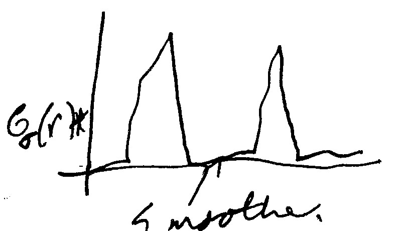
Now we have the known iris region in terms of the polar coordinates, we need to transform it into the Cartesian form. This is done with the rubber sheet model (out of scope for examination)

Paper Notes

The images of the graphs are an excerpt from my paper notes taken this session. Whilst not as good as computer generated graphs, I feel like they get the idea across well enough and strike a good balance between speed and quality.

Full paper notes for this session can be found here.

Why is a Code Needed?

For the same eye, we will get similar textures, but for a different eye, we get completely different textures. We therefore need to decompose these textures into a set of features, and we can reduce this to a texture classification problem.

Pattern Encoding

The process used in this paper makes use of 2D Gabor wavelet filters:

\[ G(\omega_0, x) = e^{-\frac{(x-x_0)^2}{2\sigma^2}} e^{i\omega_0 x} \]

Here, \(i = \sqrt{-1}\). The Gabor filter will have a real part and an imaginary part, if we decompose it from the polar representation using Euler's equation:

\[ G(\omega_0, x) = e^{-\frac{(x-x_0)^2}{2\sigma^2}} (\cos \omega_0 x + i \sin \omega_0 x) \]

This then allows us to see where the wavelet falls on a graph of \(\Re, \Im\). We can then plot a graph with \((x,\Re)\), and \((x, \Im)\). The Gabor filter used for the texture processing is a bit more complicated, as the filter introduces is the one-dimensional version.

In two dimensions, we get the imaginary and real parts, and we can encode as a phase-quadrature. Each pixel in the filter image then has a real and imaginary part. We can denote this as \(I * G = J\), where \(I\) is the image, \(*\) is a convolution, \(G\) is the Gabor filter, and \(J\) is a complex-valued output.

Given these real and imaginary parts of the output, we can plot a graph of \((\Re,\Im)\), to get the amplitude and phase of the output. We can then divide this graph into four quadrants, and for each pixel we convolve with the Gabor filter, we can assign a 2-bit code:

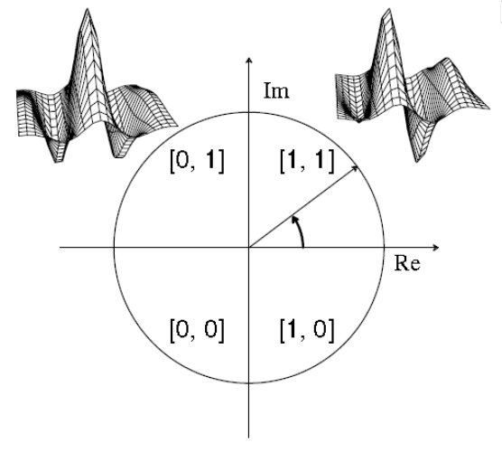
For each image of the eye, we can then run a bank of Gabor filters over it with different parameters, and encode the 2-bit demodulation code. We can repeat this until we have e.g., 2048 bits for each iris.

Hamming Distances

Given we have lots of binary codes, we need to be able to compute the similarity of two different textures. To do this, we take the Hammind distance, as a measure of the dissimilarity, and this can be done using a normalised, masked, XOR between different codes. As we're using XOR this is incredibly fast.

The Hamming distance between two eyes can be calculated using a normalised, masked XOR. In the lecture, the normalisation was explained as taking the total number of bits that matched and dividing it by the total number of bits to get the distance as a percentage, but the masking wasn't explained at all.

The equation given for the Hamming distance is as follows:

\[ HD = \frac{ || (codeA \oplus codeB) \cap maskA \cap maskB || }{ || maskA \cap maskB || } \]

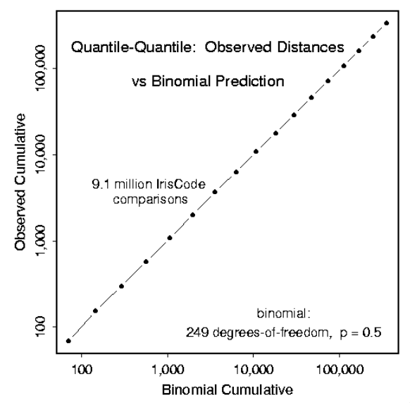
The Hamming distance between a population of irises perfectly creates a bionomial distribution around 0.5. Based on the data from the irises, we can see a one-to-one correspondence between the theoretical and actual values from the Hamming distance data, showing that we perfectly match a binomial distribution.

Recognition

For different irises, the difference is normally around 0.5. For the same person, the Hamming distance will be much closer to zero, with a slight spread due to the inherent noise from capture of the irises.

This can be seen in the graph below:

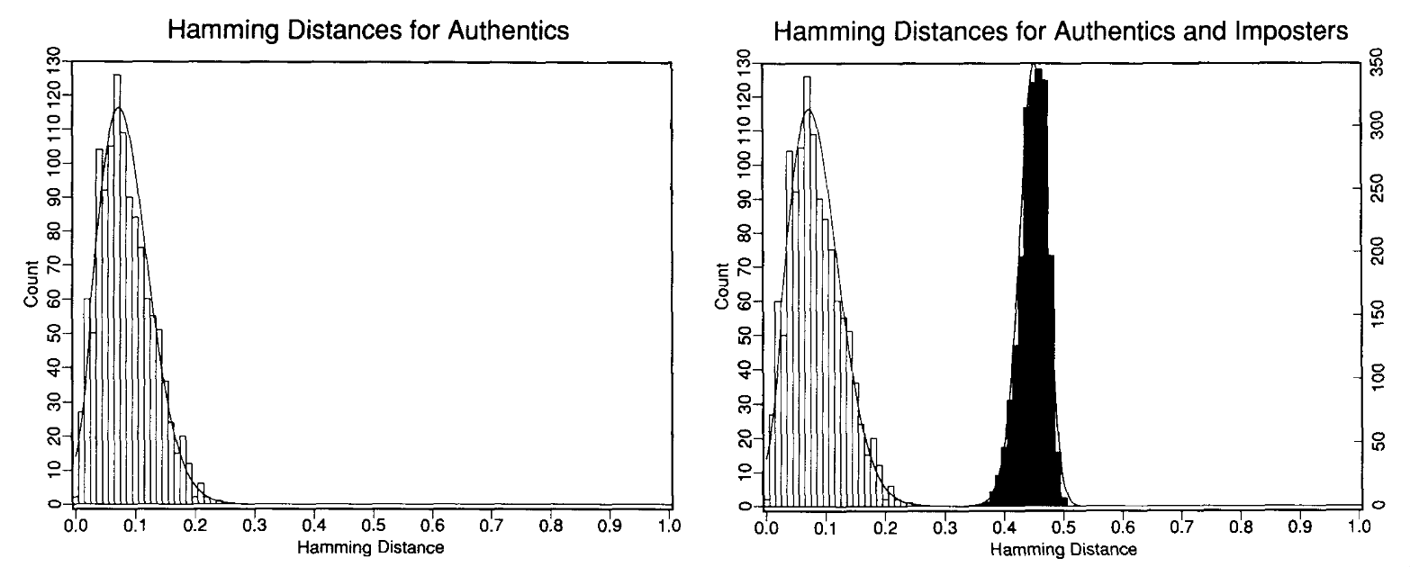
This is known as the decision environment, and is a historgram of the density versus the Hamming distance. The graph shows for a very favourable set of conditions.

In unfavourable conditions, with different distance acquisitions, by different optics, there are still two main peaks on the distribution. The highest value of the distance is still lower than the lowest value for when irises are different.

Once we know the iris codes, we can then use a KNN algorithm and a dataset of irises to calculate and classify the test data to one of the groups.

Twins

For twins, their irises are different, and we can also look at the Hamming distance between them. This is due to the difference between the genotype and the phenotype.

When doing iris matching, we need to always ensure that we are looking at the same eye, because they differ for each eye on the same person.

Applications

This biometric technique is employed in various security applications, e.g., UK immigration, access control, child identification, UAE watchlist, refugees, and at airports.

It can also be used to authenticate for military and criminal purposes.

Databases

The main datasets we can use to train models are CASIA 1, CASIA 3, Iris Challenge Evaluation (ICE), University of Bath, Multimedia University, West Virginia University (synthetic dataset).

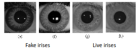
Detecting Fake vs Real Irises

For one reason or another, people may want to mask their true iris. This could be to evade police identification, or to try and trick a machine that recognises people into thinking that you are another person.

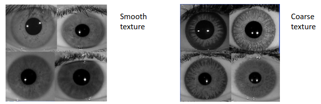
Fortunately, for us, fake irises have much sharper edges than real irises, and a much coarser texture. We can use measures from the grey-level co-occurrence to automatically see this. The main paper of interest for this is Wei, Qiu, and T Tan, ICPR 2009.

Quality Assessment

We can quantitatively get the quality of an iris, by first performing a coarse localization of the pupil. From here, we can then do a Fourier transform of the two local regions, giving two separate frequency domain plots.

For coarse localization, we take two windows either side of the pupil, which is the basis for our Fourier transform. If the iris is fake, and contains sharp edges, then the bandwidth of the Fourier transform would be wider than that for a real iris.

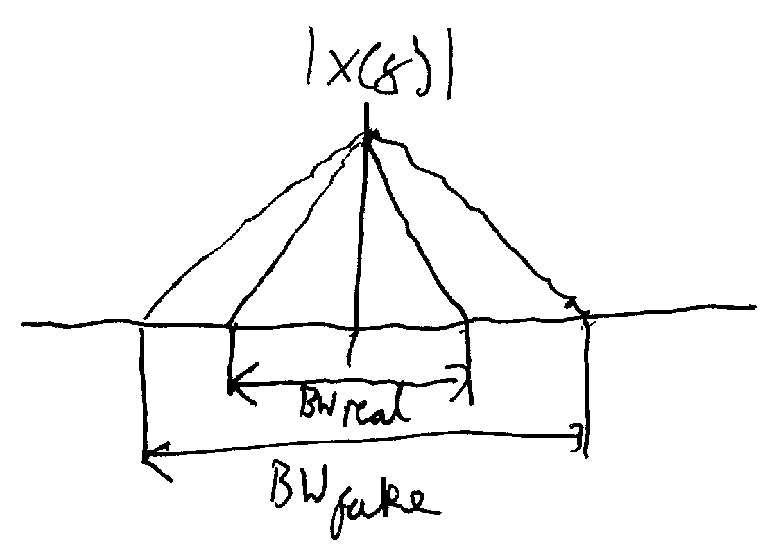
We can then take the mean of these plots and feed into a support vector machine for classification, training it in a supervised way with a set of real irises and a set of fake irises. This method was introduced by L Ma, T Tan, Y Wang, IEEE TPAMI 2003.

Active Contours

The method set out earlier in these notes attempts to find the boundary of the iris by maximising some \(r\) on a circle \(x_0,y_0\). This works well, provided that there is a clean transition period from the iris to the sclera, and that the boundary is circular.

For most irises, the boundary will be circular, but may be occluded, e.g., by the eyelids. Instead of using the method outlined above, we may instead make use of active contours to get the mask of the iris, and this mask may be non-circular. This method was proposed by J. Daugman, IEEE TSMC, 2007.

Extra Research

Would like to see how this recognition technique changes with the size of the pupil, as changes in light levels change the size of the pupil but not the iris.